“Another article comparing types of autoencoders?”, you may think. “There are already so many of them!”, you may think. “How does he know what I am thinking?!”, you may think. While the first two statements are certainly appropriate reactions - and the third a bit paranoid - let me explain my reasons for this article.
There are indeed articles comparing some autoencoders to each other (e.g. [1], [2], [3]), I found them lacking something. Most only compare a hand full of types and/or only scratch the surface of what autoencoders can do. Often you see only reconstructed samples, generated samples, or latent space visualization but nothing about downstream tasks. I wanted to know if a stacked autoencoder is better than a sparse one for anomaly detection or if a variational autoencoder learns better features for classification than a vector-quantized one. Inspired by this repository I found, I took it into my own hands, and thus this blog post came into existence.
Of course, this article will probably not be a complete list of all the autoencoders out there, there are just too many. But, if you are missing your favorite autoencoder, feel free to contact me or send a PR. I tried to structure the code to be easily extendable, and you can find it at github.com/tilman151/ae_bakeoff.
This is my first personal project with pytorch-lightning, too. It really helped to make my code more structured, readable and cut out tons of boilerplate code. You can check out this great package here.
What and how are we comparing?
First, let’s make clear what the inclusion criterion for this article is. We are interested in all modifications to a vanilla deep autoencoder that change the way the latent space behaves or may improve a downstream task. This excludes application-specific losses (e.g. perceptual VGG19 loss for images) and the types of encoder and decoder (e.g. LSTM vs. CNN). The following types have made the cut:
- Shallow Autoencoders
- Deep Autoencoders (vanilla AE)
- Stacked Autoencoders
- Sparse Autoencoders
- Denoising Autoencoders
- Variational Autoencoders (VAE)
- Beta Variational Autoencoders (beta-VAE)
- Vector-Quantized Variational Autoencoders (vq-VAE)
Aside from describing what makes each of them unique, we will compare them in the following categories:
- (Update 03.03.2021) Training time
- Reconstruction quality
- Quality of decoded samples from the latent space (if possible)
- Quality of latent space interpolation
- Structure of the latent space visualized with UMAP
- ROC curve for anomaly detection with the reconstruction error
- Classification accuracy of a linear layer fitted on the autoencoder’s features
All autoencoders tested share the same simple architecture with a fully-connected en- and decoder, batch normalization, and ReLU activation functions. The output layer features a sigmoid activation function. Save for the shallow one, all autoencoders have three encoder and decoder layers each.
The dimension of the latent space and the number of network parameters is held approximately constant. This means that a variational autoencoder will have more parameters than a vanilla one as the encoder has to produce $2n$ outputs for a latent space of dimension $n$. We make two training runs for each autoencoder: once with a latent space of 20 dimensions, and once with 2 dimensions. The model from the second training run is used for anomaly detection, the first one for all other tasks. Both variants are undercomplete, meaning that they have a higher input dimension than latent space dimension.
The MNIST dataset will serve as the venue for our contest. The default train/test split is further divided into a train/val/test split by taking a random sample of 5000 samples from the training split for validation.
Obviously, there are some limitations to what we are doing here. All training runs are only done once, so we have no measure of how stable the performances are. We are only using one dataset, so drawing any generalized conclusions is off-limits. Nevertheless, this is a blog and not a journal, so I think we are fine. With all that in mind, let’s begin our Great Autoencoder Bake Off.
The Contestants
First, we will have a look at how each tested autoencoder works and what makes them special. From that, we will try to form a few hypotheses on how they will perform on the tasks.
Shallow Autoencoder
The shallow autoencoder is not really a contestant as it is far too underpowered to keep up with the others. It is only here as a baseline.
$$\hat{x} = \operatorname{dec}(\operatorname{enc}(x))$$
Above you can see the reconstruction formula of the shallow autoencoder. The formula declares how an autoencoder reconstructs a sample $x$ in a semi-mathematical way.
A shallow autoencoder features only one layer in its encoder and decoder each. To distinguish the shallow autoencoder from a PCA, it uses a ReLU activation function in the encoder and a sigmoid in the decoder. It is therefore non-linear.
Normally, the default choice for the reconstruction loss for an autoencoder is mean squared error. We will use binary cross-entropy (BCE) because it yielded better-looking images in the preliminary experiments. If you want to know why this is a valid choice of a loss function, I recommend reading chapters 5.5 and 6.2.1 of the Deep Learning Book. As all following autoencoders, the shallow one is trained against the following version of BCE:
$$\mathcal{L}_r = \frac{1}{N}\sum_{i=1}^N \sum_{j=1}^{h\cdot w} \operatorname{BCE}(\hat{x}_j^{(i)}, x_j^{(i)})$$
where $x^{(i)}_j$ is the $j$th pixel of the $i$th input image and $\hat{x}^{(i)}_j$ the corresponding reconstruction. The loss is, hence, summed up per image, and averaged over the batch. This decision will become important for the variational autoencoder.
Deep Autoencoder
The deep autoencoder (a.k.a. vanilla autoencoder) is the big brother of the shallow one. They are basically the same, but the deep autoencoder has more layers. Therefore, they have the same reconstruction formula, too.
The deep autoencoder has no restrictions on its latent space and should, as a consequence, be able to encode the most information in it.
Stacked Autoencoder
The stacked autoencoder is a “hack” to get a deep autoencoder by training only shallow ones. Instead of training the autoencoder end-to-end, we train it in a layer-wise, greedy fashion. First, we take the first encoder and last decoder layer to form a shallow autoencoder. After training these layers, we encode the whole dataset with the encoding layer and form another shallow autoencoder from the second encoder and next-to-last decoder layer. This second shallow autoencoder is trained with the encoded dataset. This process is repeated until we arrive at the innermost layers. In the end, we get a deep autoencoder out of stacked shallow autoencoders.
We will train each of the $n$ layers for $\frac{1}{n}th$ of the total training epochs.
As the stacked autoencoder differs from a deep one only by training procedure, it has the same reconstruction function, too. Again, we have no restrictions on the latent space, but the encoding is expected to be worse due to the greedy training procedure.
Sparse Autoencoder
The sparse autoencoder imposes a sparsity constraint on the latent code. Each element in the latent code should only be active with a probability $p$. We add the following auxiliary loss to enforce it while training:
$$L_s(z) = \sum_{i=1}^N \left( p \cdot \log{\frac{p}{\bar{z}^{(i)}}} + (1 - p) \cdot \log{\frac{1 - p}{1 - \bar{z}^{(i)}}} \right)$$
where $\bar{z}^{(i)}$ is the average activation of the $i$th element of the latent code over a batch. This loss corresponds to the sum of $|z|$ Kulback-Leibler divergences between binomial distributions with the means $p$ and $\bar{z}^{(i)}$. Other implementations may be possible to enforce the sparsity constraint, too.
To make this sparsity loss possible, we have to scale the latent code to $[0, 1]$ in order to be interpreted as probabilities. This is done with a sigmoid activation function which gives us following reconstruction formula:
$$\hat{x} = \operatorname{dec}(\sigma(\operatorname{enc}(x)))$$
The complete loss for the sparse autoencoder combines the reconstruction loss and sparsity loss with an influence hyperparameter $\beta$:
$$L = L_r + \beta L_s$$
We will set $p$ to 0.25 and $\beta$ to one for all experiments.
Denoising Autoencoder
The denoising autoencoder does not restrict the latent space but aims to learn a more efficient encoding through applying noise to the input data. Instead of feeding the input data straight to the network, we add Gaussian noise as follows:
$$x’ = \operatorname{clip} (x + \mathcal{N}(0;\operatorname{diag}(\beta\mathbf{I}))) $$
where $\operatorname{clip}$ is clipping its input to $[0, 1]$ and the scalar $\beta$ is the variance of the noise. Hence, the autoencoder is trained on reconstructing clean samples from a noisy version. The reconstruction formula is:
$$\hat{x} = \operatorname{dec}(\operatorname{enc}(x’))$$
We use the noisy input exclusively in training. When evaluating the autoencoder, we feed it the original input data. Otherwise, the denoising autoencoder uses the same loss function as the ones before. For all experiments, $\beta$ is set to 0.5.
Variational Autoencoder
In theory, the variational autoencoder (VAE) has not that much to do with a vanilla one. In practice, the implementation and training are very similar. The VAE interprets the reconstruction as a stochastic process, making it non-deterministic. The encoder does not output the latent code, but the parameters of a probability distribution of latent codes. The decoder then receives a sample from this distribution. The default choice of distribution family is a Gaussian $\mathcal{N}(\mu; \operatorname{diag}(\Sigma))$. The reconstruction formula looks as follows:
$$\hat{x} = \operatorname{dec}(\operatorname{sample}(\operatorname{enc}_\mu(x), \operatorname{enc}_\Sigma(x)))$$
where $\operatorname{enc}_\mu(x)$ and $\operatorname{enc}_\Sigma(x)$ encode $x$ to $\mu$ and $\Sigma$. Both encoders share most of their parameters. In practice, a single encoder simply gets two output layers instead of one. The problem is now that sampling from a distribution is an operation without gradient and backpropagation from the decoder to the encoder would be impossible. The solution is called the reparametrization trick and transforms a sample from a standard Gaussian to one from a Gaussian parametrized by $\mu$ and $\Sigma$:
$$\operatorname{reparametrize}(\mu, \Sigma) = \Sigma \cdot \operatorname{sample}(0, \operatorname{diag}(\mathbf{I})) + \mu$$
This formulation has a gradient with respect to $\mu$ and $\Sigma$ and makes training with backpropagation possible.
The variational autoencoder further restricts the latent space by requiring Gaussian distributions to be similar to a standard Gaussian. The distribution parameters are therefore penalized with the Kulback-Leibler divergence:
$$L_{KL} = \frac{1}{2N}\sum_{i=1}^N \sum_{j=1}^{|z|} (2\Sigma_j^{(i)} + (\mu_j^{(i)})^2 - 1 - 2\log{(\Sigma_j^{(i)})})$$
The divergence is averaged over the batch. The reconstruction loss is, as mentioned before, averaged in the same way to retain the correct ratio between the reconstruction loss and the divergence loss. The full training loss is then:
$$L = L_r + L_{KL}$$
As we try to constrain the encoder to output standard Gaussians, we can try to decode a sample from a standard Gaussian directly, too. This unconditioned sampling is a unique property of VAEs and makes them generative models, similar to GANs. The formula for unconditional sampling is:
$$\hat{x} = \operatorname{dec}(\operatorname{sample}(0, \operatorname{diag}(\mathbf{I}))$$
If you want to understand the theory behind VAEs, I recommend the tutorial by Carl Doersch.
Beta Variational Autoencoder
The beta VAE is a generalization of the VAE that simply changes the ratio between reconstruction and divergence loss. The influence of the divergence loss is parametrized by a scalar $\beta$, hence the name:
$$L = L_r + \beta L_{KL}$$
A $\beta < 1$ relaxes the constraints on the latent space while a $\beta > 1$ makes the constraint stricter. The former should result in better reconstructions and the latter in better unconditional sampling. The theoretic derivation makes good arguments about what else this simple change affects. You can read them on OpenReview. We will use a strict version of this autoencoder with $\beta = 2$ and a loose version with $\beta = 0.5$.
Vector-Quantized Variational Autoencoder
The vector-quantized variational autoencoder (vq-VAE) is a VAE that uses a uniform categorical distribution to generate its latent codes. Each element of the encoder output is replaced by the categorical value of the distribution that is its nearest neighbor. This is a form of quantization and means that the latent space is not continuous anymore but discrete.
$$\hat{x} = \operatorname{dec}(\operatorname{quantize}(\operatorname{enc}(x))))$$
The categories themselves are learned by minimizing the sum squared error to the encoder outputs:
$$L_{vq} = \frac{1}{N}\sum_{i=1}^N \sum_{j=1}^{|z|} (\operatorname{sg}(z_j^{(i)}) - \hat{z}_j^{(i)})^2$$
where $z$ is the output of the encoder, $\hat{z}$ is the corresponding quantized latent code, and $sg$ the stop gradient operator. On the other hand, the encoder is encouraged to output encodings similar to the categories by sum squared error, too:
$$L_{c} = \frac{1}{N}\sum_{i=1}^N \sum_{j=1}^{|z|} (z_j^{(i)} - \operatorname{sg}(\hat{z}_j^{(i)}))^2$$
This is called the commitment loss. A Kulback-Leibler divergence loss is not necessary, as the divergence would be a constant for a uniform categorical distribution. Both losses are combined with the reconstruction loss by a hyperparameter $\beta$ controlling the influence of the commitment loss:
$$L = L_r + L_{vq} + \beta L_c$$
We set $\beta$ to one for all experiments.
Because the vq-VAE is a generative model, we can sample from it unconditionally, too. In the original paper, a pixel-CNN is used to autoregressively sample a latent code. For simplicity’s sake, we will sample by drawing categories uniformly.
The Gauntlet
Now that we know who we are dealing with, let’s see how they fare in our gauntlet of tasks. Besides the standard ones like reconstruction quality, we will have a look at semi-supervised classification and anomaly detection, too.
Training Time
(Update 03.03.2021) As per feedback from Reddit, we are going to look at the training times of the autoencoders. The time was not recorded directly because we would need to rerun the experiments to do that. Instead, we are using the TensorBoard event files and calculate the time between the first training loss and last validation loss logged. This gives us only an offset of the iteration time of the first training batch. The times should, therefore, be interpreted as the time to run 60 epochs with validation after each one.
| shallow | vanilla | stacked | sparse | denoising |
|---|---|---|---|---|
| 0:10:38 | 0:11:15 | 0:11:05 | 0:11:27 | 0:11:18 |
| vae | beta_vae_strict | beta_vae_loose | vq |
|---|---|---|---|
| 0:11:30 | 0:11:29 | 0:11:28 | 0:11:27 |
Unsurprisingly, there is not much of a difference. Even the shallow autoencoder, that is much smaller, takes only about half a minute less time. This indicates that the time for the forward and backward passes is much smaller than the overhead of data loading, logging, etc. Some variation can be attributed to this being computed on a Windows machine, too. Who knows what background process is hogging resources at any given time?
Reconstruction
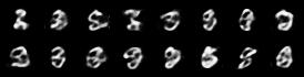
First and foremost, we want to see how well each autoencoder can reconstruct its input. For this, we can have a look at the 16 first images of the MNIST test set.
| shallow | vanilla | stacked | sparse | denoising |
|---|---|---|---|---|
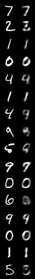 | 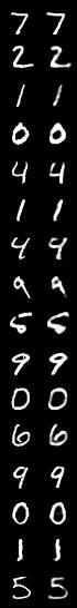 | 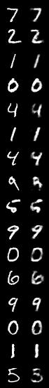 | 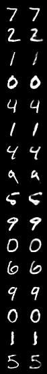 | 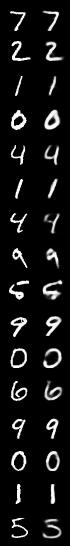 |
| vae | beta_vae_strict | beta_vae_loose | vq |
|---|---|---|---|
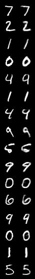 | 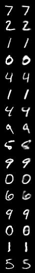 | 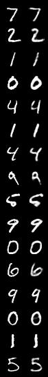 | 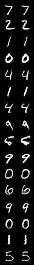 |
The shallow autoencoder fails to reconstruct many of the test samples correctly. Fours and nines are barely distinguishable, and some digits are not recognizable at all. The other autoencoders do a much better, but not perfect, job. The denoising one is in the habit of making some thin lines disappear. The sparse and stacked ones seem to have problems with abnormally formed digits like the five and one of the nines. Overall the reconstructions are a little blurry, which is normal for autoencoders. The vq-VAE produces slightly less blurry reconstructions, which the original authors credit to the discrete latent space.
Otherwise, there is little difference to be seen between the different autoencoders. This is supported by the reconstruction errors over the whole test set. The table below lists the summed binary cross-entropy averaged over the samples of the set.
| shallow | vanilla | stacked | sparse | denoising |
|---|---|---|---|---|
| 123.2 | 63.92 | 87.87 | 64.27 | 75.15 |
| vae | beta_vae_strict | beta_vae_loose | vq |
|---|---|---|---|
| 76.12 | 86.12 | 69.51 | 64.49 |
Trailing far behind, as suspected, is the shallow autoencoder. It simply lacks the capacity to capture the structure of MNIST. The vanilla autoencoder fares comparatively well, securing 1st place together with the sparse autoencoder and the vq-VAE. Both of the latter do not seem to suffer from their latent space restrictions in this regard. The VAE and beta-VAEs, on the other hand, do achieve a higher error, due to their restrictions. Besides, the sampling process in the VAEs introduces noise that harms the reconstruction error.
We will see later if reconstruction ability is a good proxy of performance on the other tasks.
Sampling
The next trial will be a bit shorter, as only four contestants can sample unconditionally from their latent space: VAE, loose and strict beta-VAE, as well as vq-VAE. For each of them, we sample 16 latent codes and decode them. For the VAE and beta-VAEs, we sample from a standard Gaussian. The latent codes for the vq-VAE will be sampled uniformly from their learned categories.
| vae | beta_vae_strict |
|---|---|
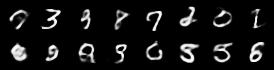 |  |
| beta_vae_loose | vq |
|---|---|
 |  |
None of them look pretty, but we can glance at some differences, nonetheless. The most meaningful samples were generated by the strict beta-VAE. This was expected because its training laid the highest emphasis on enforcing the Gaussian prior. Its encoder output is therefore most similar to samples from a standard Gaussian which enables the decoder to successfully decode latent codes sampled from a true standard Gaussian.
The variance of images on the other hand is relatively small. We can see many fiveish, sixish-looking digits on the right, for example. The loose variant offers more diverse generated images, even though, less of them are legible. This makes sense, as the loose beta-VAE laid less emphasis on the prior and could encode more information into the latent space. Then again, it’s encoder outputs are less similar to standard Gaussian samples, which is why it fails to assign the unconditioned samples any meaning most of the time. The standard VAE lays somewhere between the other two, which is no surprise here.
A bit of a disappointment is the sampled images from the vq-VAE. They do not resemble MNIST digits at all. The vq-VAE does not seem to support easy sampling by uniformly drawing categories and a more complex, learned prior seems, indeed, necessary.
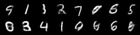
Interpolation
The interpolation task shows us how densely the regions of the latent space are populated. We encode the first two images from the test set, a two and a seven, and interpolate linearly between them. The interpolations are then decoded to receive a new image. If the images from the interpolated latent codes show meaningful digits, the latent space between the class regions was effectively used by the autoencoder.
For all VAE types, we interpolate before the bottleneck operation. This means that we interpolate the Gaussian parameters and then sample from them for the VAE and beta-VAE. For the vq-VAE, we first interpolate and then quantize.
| shallow | vanilla | stacked |
|---|---|---|
 |  |  |
| sparse | denoising | vae |
|---|---|---|
 |  |  |
| beta_strict | beta_loose | vq |
|---|---|---|
 |  |  |
Above you can see GIFs looping through the interpolated images back and forth, briefly stopping at the original images. We can see that the VAE and beta-VAEs produce relatively meaningful interpolations, going from a two over something looking threeish to a seven. The jitter you see is an artifact of the sampling process in the bottleneck. It could be avoided through the reparametrization trick, where we could sample only once from the standard Gaussian for the whole interpolation process.
The rest of the autoencoders do not seem to produce meaningful interpolations at all. They simply fade out pixels not needed and fade in new ones, while the VAE seems to bend the digit from one class to the other. Even though the vq-VAE is a VAE in theory and name, too, it does not show this property. Why the interpolation of the vq-VAE looks more like the vanilla one than the other VAE ones, becomes apparent when looking at the latent space.
Latent Space Structure
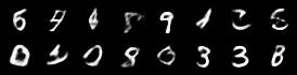
We are talking about the latent space a lot in this article, but how does it look like? Unfortunately, conceptualizing a 20-dimensional space in our mind is not a task humans were designed for at all, but there are tools at our disposal that let us overcome this hurdle. The UMAP algorithm is the go-to tool when it comes to visualizing high-dimensional spaces. It can reduce the latent space to two dimensions while preserving the neighborhood of the latent codes. Why look at the latent space of an autoencoder with two dimensions when you can have a pretty accurate representation of a 20-dimensional one? In the picture below, you can see a scatter plot for each of our autoencoders’ latent spaces. Each point is the latent code for one image from the test set and the color represents the digit in the image. The scales of the x- and y-axis don’t have any specific meaning.
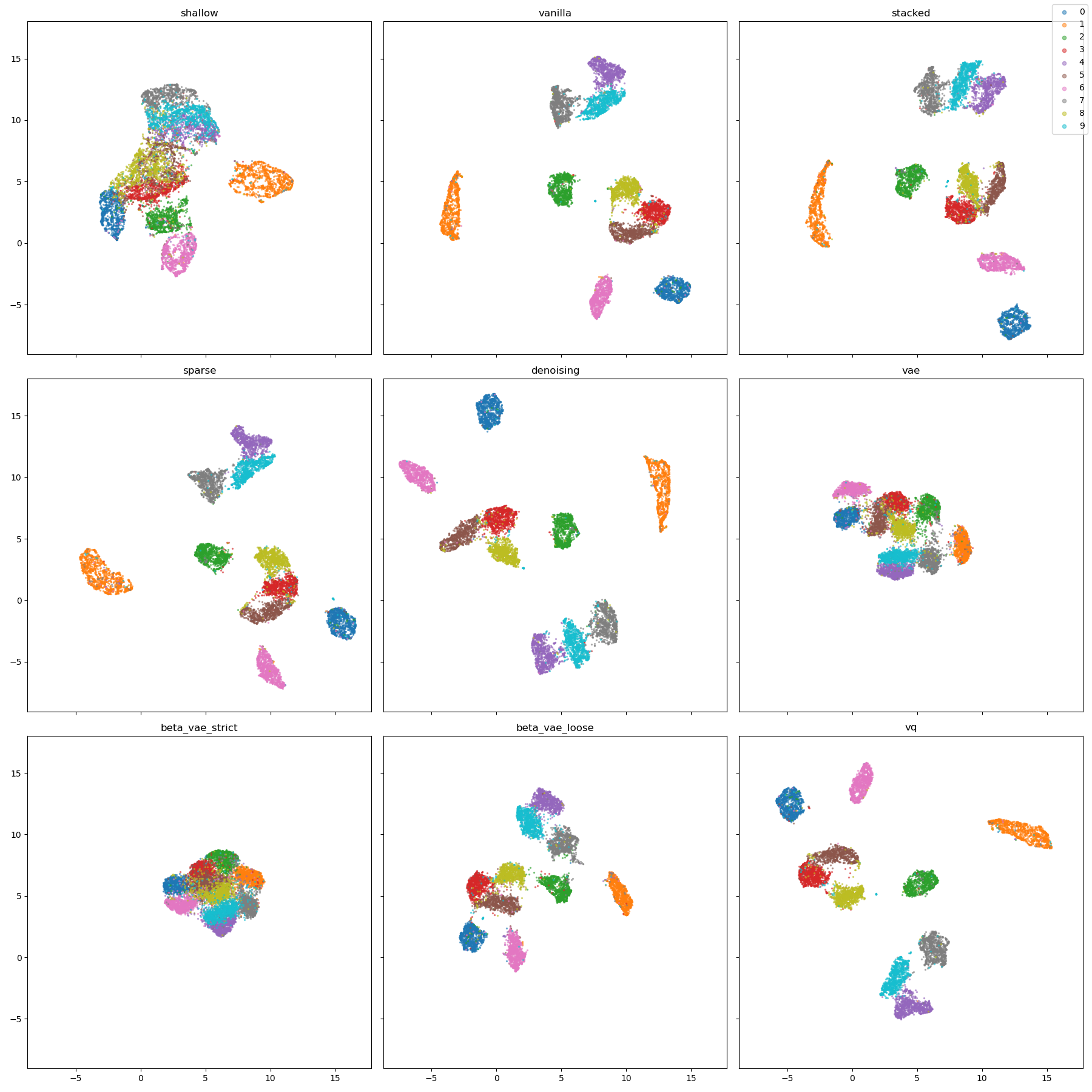
There are some obvious similarities between the plots. First of all, we can see that the plots of vanilla, stacked, sparse, denoising, and vq-VAE are quite similar if we ignore different rotations. The clusters of zeros (blue), ones (orange), twos (green), and sixes (pink) are always nicely separated, so they seem to be quite different from the other digits. Then, we have a cluster of 4-7-9 (purple-gray-turquoise) and a cluster of 3-5-8 (red-brown-yellow). This hints at a connection between these digits, e.g swap the upper vertical line of a three and you get a five, add two more vertical lines and you get an eight. The autoencoders seem to encode the structural similarities between the digits.
The shallow autoencoder seems to struggle to separate the digits into clusters. While the cluster of ones is nicely separated, the other digits’ clusters are overlapping. This means that the shallow autoencoder maps some instances of different digits to the same latent code, leading to weird results we have seen in the reconstructions.
The plots of the VAE and beta-VAEs seem quite different from the others. Here we can see the influence of the divergence loss really well. The latent codes occupy less space than the other autoencoders’ codes because the divergence loss restricts them to be samples of a standard Gaussian. The strict beta-VAE uses the least space because the divergence loss is enforced the most.
We can explain the interpolation behavior of the VAEs, too. The VAE and strict beta-VAE produce something looking like a three during the interpolation, while the loose beta-VAE does not. For both of the former, the clusters of two (green) and three (red) are neighbors and are completely separated for the latter. It seems plausible that we may pass the border of the cluster of threes during interpolation.
As mentioned before, the latent space of the vq-VAE looks much more like the vanilla one’s than the latent space of the other VAEs. This seems to be a plausible explanation for why the interpolations of the vq-VAE look like the ones of the vanilla autoencoder.
Classification
Ok, so looking at generated images and latent spaces is nice and all, but what if we want to do something productive with an autoencoder? The latent space plots have shown us that some autoencoders are quite good at separating the digit classes in MNIST, although they did not receive any labels. Let’s take a look at how we can leverage this finding for classifying the MNIST digits.
We will use the 20-dimensional latent codes from our trained autoencoders and fit a dense classification layer on it. The layer will be trained on only 550 labeled samples of the training set against cross-entropy. In other words, we are using our autoencoders for semi-supervised learning. For comparison, training the vanilla encoder plus classification layer from scratch yields an accuracy of $0.4364$. We will see if our autoencoders can improve on that in the table below.
| shallow | vanilla | stacked | sparse | denoising |
|---|---|---|---|---|
| 0.4511 | 0.7835 | 0.6107 | 0.2221 | 0.8049 |
| vae | beta_vae_strict | beta_vae_loose | vq |
|---|---|---|---|
| 0.6016 | 0.4536 | 0.6311 | 0.7717 |
Unsurprisingly, nearly all autoencoders improved on the baseline, with the sparse one being the exception. The denoising autoencoder takes the first place, closely followed by the vanilla autoencoder and vq-VAE. It seems that the added input noise of the denoising autoencoder produces features that generalize best for classification.
The most interesting is in my opinion, that even the shallow autoencoder slightly improves the accuracy, even though it has only one layer and much fewer parameters. This shows once again that intelligent data usage often beats bigger models.
The VAE and beta-VAE show again how the divergence loss restricts the latent space. The loose beta-VAE achieves the highest accuracy as it can encode much more information than the other two. An interesting use case would be sampling multiple latent codes and classifying them. This could give a better measure of classification uncertainty. A quick Google search did not yield any papers on this, but it would be weird if nobody tried this already.
The results of the sparse autoencoder warrant a closer inspection, as they are much worse than the baseline. It seems that sparse features are not suited for classifying MNIST at all. We would need to test the sparse autoencoder on other datasets to see if it works better.
Anomaly Detection
In anomaly detection, or novelty detection to be specific, we want to find outlier samples in our test data, given our training data has no such outliers. Common applications are network intrusion detection or fault detection in predictive maintenance. We will fabricate an anomaly detection task from MNIST by excluding all images of ones from the training data. Afterward, we will see if the trained model can separate the ones in the test set from the other digits.
Doing anomaly detection with autoencoders is relatively straight-forward. We take the trained model and calculate the reconstruction loss for our test samples. This is our anomaly score. If the reconstruction of a sample is good, it is probably similar to the training data. If the reconstruction is bad, the sample is considered an outlier. The autoencoder is expected to exploit correlations between features of the training data to learn an effective, low-dimensional representation. As long as these correlations are present, a test sample can be reconstructed quite well. If any of the correlations are not holding for a test sample, the autoencoder will fail to reconstruct it, to a degree.
An obvious challenge for this task is to find the optimal threshold for the anomaly score to consider a sample an anomaly. We will leave this problem for someone else to solve (as most publications do, too) and report the ROC plot and the area under the curve (AUC).
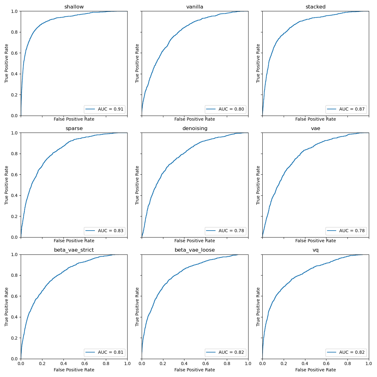
The results of this last task came as a bit of a surprise for me. I did some digging for bugs, but I am sure now that they are valid. The shallow autoencoder leaves all other autoencoders in the dust with a whooping $0.91$ AUC. Up next would be the stacked autoencoder with a narrow field of the remaining ones behind it. This order is stable for different digits and dimensions of the latent space, too.
So, why is that? How are the two autoencoders that trailed behind in almost all other tasks so good at anomaly detection? It seems that all other tasks rely on how well the learned latent space is able to generalize. The better it is at that, the better you can classify on it, the better you can reconstruct unseen samples. This time we do not want to generalize. At least not too well. We rely on the fact that samples too dissimilar to the training data cannot be reconstructed. If our latent space generalizes too well, we are hurting our anomaly detection performance.
The ability of an autoencoder to generalize is dependent on its encoder and decoder capacity, as well as the dimensionality of the latent space. We already lowered the dimensionality of the latent space to two for the anomaly detection, so there is not much room to go lower. Through its limited capacity, the shallow autoencoder struck the right balance of how well it modeled the training data. The stacked autoencoder’s greedy layer-wise training is limiting its ability to generalize similarly.
In the end, we may have to conclude that MNIST is just too damn easy. The deep autoencoders have much more capacity than it is helpful for this dataset. Of course, there are other perspectives, too. We could argue that images of ones are well within the domain of the training data, as it is a digit, too. The choice of our anomaly class was completely arbitrary. Maybe another autoencoder would have been most successful in separating digits from letters, but all this is a topic for another time.
Conclusion
What a ride! We had our hypotheses confirmed, our latent spaces visualized and, finally, our expectations subverted. Do we have a conclusive champion of autoencoders? No, we do not. In the end, it is, again, a matter of the right tool for the job. You want to generate faces from noise? Use a variational autoencoder. They are too blurry? Try the vq-VAE with a learned prior. Classification? The denoising autoencoder seems fine. If you are doing anomaly detection, maybe try a shallow one first or even PCA. Sometimes less is better.
As I said in the beginning, this article cannot draw any conclusions beyond MNIST, but it serves as a good pointer, nevertheless. It would be interesting to do another run with a more complex dataset or one where the sparse autoencoder had its time to shine. A more focused look at what goes on in anomaly detection would be a nice thing, too.
As always, more questions generated than answered.